Does Better Embedding Quality Actually Improve Bayesian Optimization with LLMs?
2026-04-22
A systematic investigation into BOPRO for molecular optimization
Introduction
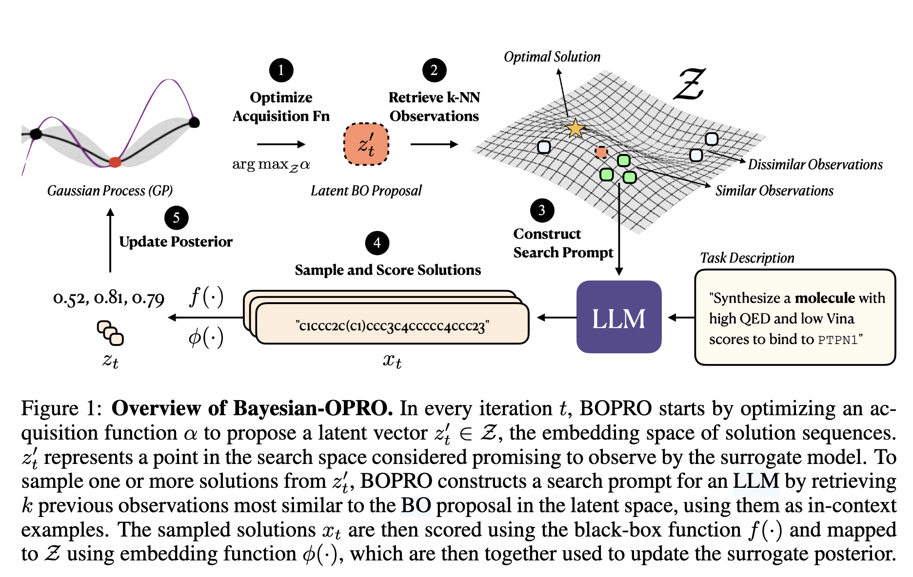
Last year, Agarwal et al. published BOPRO (ICLR 2025), a clever algorithm that combines Bayesian optimization with LLM-based search. The idea is elegant: instead of searching directly in the space of solutions, BOPRO (1) optimizes an acquisition function over a Gaussian Process (GP) surrogate to propose a promising latent vector, (2) retrieves the k-nearest neighbors of that vector in embedding space as in-context examples, (3) constructs a prompt and asks an LLM to generate new candidate solutions, (4) scores those candidates with the black-box objective, and (5) updates the GP posterior with the new observations.
It's an elegant division of labor: the GP handles principled exploration of the solution space, while the LLM provides the domain knowledge to generate valid, coherent candidates the GP could never propose on its own. Figure 1 from the paper illustrates the full loop:
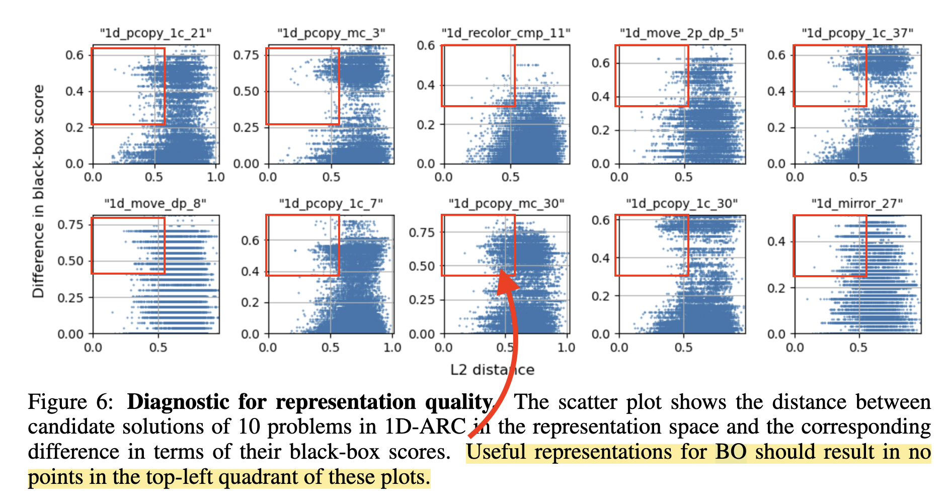
The paper identifies a key failure mode: when the embedding function is poor the GP surrogate is wrong, and the whole approach breaks down. What does poor mean? When nearby points in latent space don't have similar objective values. They show a striking diagnostic (Figure 6) for the 1D-ARC task: points that are close in embedding space have wildly different scores, violating the GP's smoothness assumption. This means step (1) is broken: the acquisition function is optimizing over a surrogate that has no reliable signal, so the latent vector it proposes is essentially random, and the k-NN examples retrieved in step (2) are uninformative.
This failure mode is real. But the paper never systematically asks: what happens if we fix the embeddings? For molecular optimization specifically, they use Molformer embeddings without ever showing the diagnostic plot.
I decided to investigate.
The Setup: Dockstring Molecule Optimization
The task is multi-target molecular optimization using Dockstring: find SMILES strings that maximize a scalarized combination of drug-likeness and binding affinity across protein targets. Of the 58 available targets in Dockstring, I used 23 total: 13 as training targets to collect fine-tuning data, and 10 held out exclusively for BOPRO evaluation. The fine-tuning model never sees molecules scored against the test targets. Budget: 200 molecules per test target.
The two components of the score are:
- QED (Quantitative Estimate of Druglikeness): a summary statistic of a molecule's drug-like properties (molecular weight, solubility, number of hydrogen bond donors/acceptors, etc.) Ranges from 0 to 1; higher is more drug-like.
- AutoDock Vina score: a physics-based docking simulator that estimates how tightly a molecule binds to a target protein's active site. More negative = stronger predicted binding. We negate and normalize it (NNV) so that higher is better.
Following the paper, the scalarized objective is 0.2 × QED + 0.8 × NNV, weighted toward binding affinity since that's the harder and more target-specific part of the problem.
I used Molformer (IBM's 47M-parameter molecular transformer) as the base embedding model, following Agarwal et al. For the LLM, I used Claude Sonnet 4.6 — a stronger model than the paper's Mistral-Large. As we'll see, that choice turns out to matter a lot.
Phase 1: Does the Embedding Bottleneck Exist for Molecules?
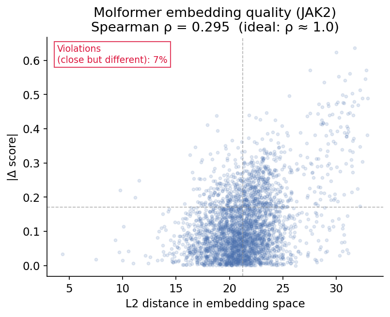
First, I reproduced the paper's diagnostic on Molformer embeddings. I scored ~500 molecules from ZINC250k (a standard benchmark set of ~250,000 drug-like molecules) against each of the 10 held-out protein targets using AutoDock Vina. Each molecule gets a target-specific score, meaning how well it binds to that particular target protein. Then, for each target, I took every pair of scored molecules and computed two things: their L2 distance in Molformer embedding space, and the absolute difference in their binding scores. If the embeddings are good for BOPRO, these should correlate — pairs that are close in embedding space should also have similar binding affinity to the target.
Result: Spearman ρ = 0.161 across 10 test targets (avg ρ). Many pairs that are close in embedding space have large score differences. This is exactly the violation the paper warns about. The scatter plot below shows a representative example (JAK2, a kinase protein target, where we got ρ = 0.295): each point is one of 3,000 randomly sampled molecule pairs, with their embedding distance on the x-axis and their score difference on the y-axis. The pattern is consistent across all targets.
What does this mean practically? When the GP proposes a latent vector via its acquisition function, it retrieves the -nearest neighbors in embedding space as in-context examples for the LLM. If those neighbors have wildly different scores despite being "close" in embedding space, the GP is essentially pointing the LLM at random molecules. The LLM gets poor examples, and the whole search degrades toward random exploration.
This confirms the bottleneck exists for molecules. The GP surrogate is working with misleading embedding geometry.
Phase 2: Can We Fix It? Contrastive Fine-Tuning
The natural fix: fine-tune the embedding function with a score-aware contrastive loss that pulls molecules with similar scores together and pushes dissimilar-scoring molecules apart.
I used a score-weighted InfoNCE (Noise-Contrastive Estimation) loss. InfoNCE is a contrastive learning objective that trains an encoder to pull "positive" pairs together and push "negative" pairs apart in embedding space. In the standard formulation, positives are augmented views of the same input (used in self-supervised vision models like SimCLR). Here, I define positives as molecule pairs with similar binding scores, so the loss teaches the encoder that chemically similar-scoring molecules should live nearby in embedding space:
where positive pairs are molecule pairs with similar objective scores (), is a temperature parameter, and is cosine similarity.
Intuitively, the loss asks: for a given molecule , how much of the "probability mass" in embedding space is concentrated on its similarly-scoring neighbors, versus all other molecules in the batch? If the encoder is doing its job, should be close to the of molecules with similar scores, making the numerator large relative to the denominator. Minimizing the negative log pushes the encoder toward this geometry. Molecules with very different scores act as negatives and get pushed apart.
Mixed-batch fine-tuning: Train on all 13 training targets together, mixing molecules from different targets in each batch. Result: ρ improved from 0.161 to 0.284, but BOPRO performance dropped slightly (0.829 → 0.821, −1.1%).
The culprit: cross-target contamination. A molecule that binds well to EGFR (a cancer-related kinase) and a molecule that binds well to DRD2 (a dopamine receptor) might both score 0.6 on their respective targets. The loss treats them as a positive pair and pulls their embeddings together. But they're chemically optimized for completely different binding pockets. The batch mixes apples and oranges.
The fix: per-target fine-tuning. Run InfoNCE independently per target, so cross-target molecules never appear in the same loss computation. This eliminates the contamination entirely. Result: ρ improved from 0.161 to 0.348, and BOPRO performance improved slightly (0.829 → 0.831, +0.2%).
The methodological insight: cross-target batch contamination matters. If you're training a score-aware embedding for optimization, you must train per-target or risk corrupting within-target geometry.
But +0.2% is tiny. We doubled embedding quality and barely moved the needle. Why?
The Surprise: Dimensionality Was the Real Problem
I had a hypothesis: even with better embedding geometry, the GP might not be able to exploit it. A standard GP with a squared-exponential kernel in 768 dimensions is fundamentally broken. With only 200 observations, the curse of dimensionality means almost all pairwise distances concentrate around the same value. The kernel degenerates toward a constant. Fine-tuning improved the geometry of those distances but couldn't fix the dimensionality problem.
The fix: PCA. Reduce the 768D embeddings to 32D or 64D before GP fitting. PCA is fit on the ~2,500 cached molecules per target at run start. The GP, acquisition function, and k-NN retrieval all operate in the reduced space.
Results across 10 targets, 3 runs each:
| Condition | GP dim | Mean best score | Targets improved | Δ vs baseline |
|---|---|---|---|---|
| Baseline Molformer | 768 | 0.829 | — | — |
| Per-target fine-tuned | 768 | 0.831 | 5/10 | +0.002 |
| Baseline + PCA-32 | 32 | 0.829 | 5/10 | +0.004 |
| Baseline + PCA-64 | 64 | 0.835 | 6/10 | +0.011 |
| Per-target fine-tuned + PCA-32 | 32 | 0.833 | 6/10 | +0.008 |
PCA-64 baseline beats everything, including the carefully fine-tuned model. A five-line sklearn call outperforms weeks of contrastive training on a GPU. The GP can actually use the lower-dimensional space — distances are spread out, the kernel is non-degenerate.
But notice: the best improvement is still only +1.1%. Even with the dimensionality problem fixed, BOPRO barely improves.
Is the GP Doing Anything at All?
This raises a harder question. The BOPRO loop uses the GP in two ways: (1) to propose a latent vector via the acquisition function to guide where to explore, and (2) to select which -neighbors to retrieve as in-context examples for the LLM. If the LLM has such a strong chemistry prior that it generates good molecules regardless of which examples it sees, the GP might be nearly irrelevant.
To test this, I ran two ablations across all 10 targets, 3 runs each:
- OPRO-greedy: Skip the GP entirely. At each step, show the LLM the -highest-scoring molecules seen so far. No acquisition function, no embedding-guided retrieval — pure greedy exploitation.
- Random-k: Show the LLM -randomly selected molecules from the observation history. No scoring, no GP.
The results were the most striking of the entire project:
| Condition | Mean best score | Targets beating BOPRO |
|---|---|---|
| BOPRO (GP + embeddings) | 0.825 | — |
| OPRO-greedy (no GP) | 0.843 | 8/10 |
| Random-k (no GP, random) | 0.825 | 5/10 |
OPRO-greedy — which has no GP, no acquisition function, and no embeddings — beats BOPRO on 8 out of 10 targets with a +2.2% mean improvement. Random-k exactly matches BOPRO.
Per-target breakdown:
| Target | BOPRO | OPRO-greedy | Random-k |
|---|---|---|---|
| MAPK1 | 0.829 | 0.830 | 0.805 |
| SRC | 0.779 | 0.821 | 0.829 |
| JAK2 | 0.845 | 0.886 | 0.823 |
| KIT | 0.823 | 0.834 | 0.828 |
| PPARA | 0.798 | 0.795 | 0.851 |
| AR | 0.815 | 0.822 | 0.835 |
| DRD2 | 0.896 | 0.923 | 0.901 |
| ADRB1 | 0.848 | 0.879 | 0.850 |
| MMP13 | 0.877 | 0.877 | 0.861 |
| CASP3 | 0.738 | 0.760 | 0.672 |
| Mean | 0.825 | 0.843 | 0.825 |
This result implies two things:
The GP acquisition function is not helping; it may be actively harmful. BOPRO uses Log Expected Improvement (LogEI) as its acquisition function: a standard Bayesian optimization criterion that scores each point in latent space by how much improvement over the current best score it is expected to deliver, according to the GP surrogate. The idea is to balance exploration (regions of high uncertainty) and exploitation (regions the GP predicts are good). But with a broken 768D GP, the surrogate's predictions are unreliable, so LogEI is proposing latent vectors in regions the model thinks are promising but aren't. OPRO-greedy sidesteps this entirely by just asking the LLM to improve on the best solutions found, which turns out to be a better strategy.
Showing the LLM good examples matters, but the GP isn't needed to find them. Random-k matches BOPRO exactly (0.825), confirming that the GP's exploration isn't finding better neighborhoods than chance. But OPRO-greedy beats random by +2.2% — so which examples you show the LLM does matter. Showing the best-scoring molecules as in-context examples is a stronger signal than GP-guided retrieval. The LLM learns "make something like these, but better" more effectively from high-quality examples than from geometrically proximal ones.
This reframes the whole BOPRO story for molecules: the LLM is doing the optimization, and the GP is getting in the way.
Does LLM Quality Change the Picture?
The original BOPRO paper used Mistral-Large, a much weaker model than what I used (Claude Sonnet 4.6). A natural objection: maybe the GP is genuinely useful with a weaker LLM, and our Sonnet results are a special case.
To test this, I re-ran all three conditions using Claude Haiku 4.5 — a significantly weaker model — on 5 representative targets.
| Target | Sonnet BOPRO | Sonnet OPRO | Haiku BOPRO | Haiku OPRO | Haiku Random |
|---|---|---|---|---|---|
| MAPK1 | 0.829 | 0.830 | 0.762 | 0.787 | 0.781 |
| JAK2 | 0.845 | 0.886 | 0.801 | 0.795 | 0.769 |
| DRD2 | 0.896 | 0.923 | 0.722 | 0.745 | 0.835 |
| CASP3 | 0.738 | 0.760 | 0.605 | 0.631 | 0.580 |
| SRC | 0.779 | 0.821 | 0.704 | 0.779 | 0.708 |
| Mean | 0.817 | 0.844 | 0.719 | 0.748 | 0.735 |
OPRO-greedy beats BOPRO with Haiku too (+4%). The hypothesis that the GP would help with a weaker LLM didn't hold. The GP underperforms OPRO-greedy regardless of LLM quality at this budget.
LLM quality has a massive effect on absolute scores. Haiku averages ~0.10 below Sonnet across all conditions — a gap larger than every embedding intervention we tried combined. Upgrading your LLM does more for molecular optimization performance than improving your GP surrogate.
The reason OPRO-greedy still wins with Haiku: even a weak LLM benefits more from seeing the best examples found so far than from GP-guided neighborhood exploration. The GP's noise in 768D is harmful regardless of whether the LLM can exploit better regions.
Putting It All Together
Here's the complete picture across all conditions (Sonnet, 10 targets):
| Condition | Mean score | Δ vs BOPRO |
|---|---|---|
| BOPRO baseline (768D GP) | 0.825 | — |
| BOPRO + per-target fine-tuned embeddings | 0.831 | +0.7% |
| BOPRO + PCA-32 | 0.829 | +0.5% |
| BOPRO + PCA-64 | 0.835 | +1.2% |
| BOPRO + per-target fine-tuned + PCA-32 | 0.833 | +1.0% |
| Random-k (no GP) | 0.825 | 0.0% |
| OPRO-greedy (no GP) | 0.843 | +2.2% |
| Switch Sonnet → Haiku (any method) | ~0.72 | −12% |
The best BOPRO improvement from any architectural change is +1.2% (PCA-64). Switching from Sonnet to Haiku costs −12%. LLM quality is an order of magnitude more impactful than GP design at this budget.
What We've Learned
1. The embedding bottleneck is real but the wrong thing to fix. Yes, Molformer embeddings violate GP smoothness (ρ=0.161). The paper's diagnosis is correct. But fixing the embedding geometry via fine-tuning or PCA barely moves BOPRO performance (+0.2% to +1.2%). The bottleneck isn't primarily the embedding.
2. The GP itself is the bottleneck at this budget. OPRO-greedy beats every embedding intervention by a wide margin, and does so with both strong and weak LLMs. The GP acquisition function, even when given better-structured input, is not reliably guiding exploration toward better regions. With 200 observations in 768D space, the surrogate model is too uncertain to be useful.
3. GP dimensionality matters more than embedding quality, but not as much as dropping the GP. PCA-64 (+1.2%) beats fine-tuning (+0.7%), confirming that distance concentration in 768D is a real problem. But even fixing dimensionality doesn't match simply removing the GP (+2.2%).
4. Per-target InfoNCE is the right way to train score-aware embeddings. Mixed-batch InfoNCE (Exp 3.1) actively hurts (−1.1%) due to cross-target gradient contamination. If you use contrastive fine-tuning for BO, train within-target.
5. LLM quality dominates everything else. The Sonnet vs Haiku gap (−12%) dwarfs every GP or embedding intervention. The in-context examples matter for guiding the LLM (OPRO-greedy > random), but the LLM's underlying capability is the primary driver of optimization performance.
Implications
For practitioners using BOPRO or similar LLM+BO hybrids:
- Try OPRO-greedy first. It's simpler, faster (no GP fitting), and in our experiments outperforms the full BOPRO loop with both strong and weak LLMs at a 200-molecule budget.
- If you need the GP: Use PCA-64 before fitting. It's a free +1.2% improvement that addresses distance concentration in high-dimensional embedding spaces.
- If you fine-tune embeddings: Train per-target. Mixed-batch training with a scalarized multi-objective score corrupts within-target geometry.
- Invest in your LLM first. The Sonnet vs Haiku gap (−12%) dwarfs any GP or embedding optimization. If you have a fixed compute budget, a better LLM will outperform a better surrogate model.
The broader lesson: when an LLM is part of a hybrid optimization loop, it may dominate the learned surrogate — especially at small data budgets. The GP's value is as an exploration mechanism, but with 200 observations in 768D space the surrogate is too uncertain to guide useful exploration. At larger budgets, the balance may shift.
Limitations and Future Work
- Budget: 200 molecules per target. GP quality may matter more at larger budgets (500–1000 evaluations) where the surrogate accumulates enough data to be reliable, and where OPRO-greedy's greedy exploitation may plateau.
- LLM range: We tested Sonnet 4.6 (strong) and Haiku 4.5 (weak) — both show OPRO-greedy > BOPRO. Testing with Mistral-Large (the paper's original model) would be the most direct comparison to the paper's setting.
- Single embedding model: Molformer is good but not state-of-the-art. A better task-specific encoder (e.g., Uni-Mol) might change the embedding story.
- Fine-tuning + PCA-64: We only evaluated the per-target fine-tuned embedding with PCA-32. The combination with PCA-64 is untested and may stack the two improvements.
- OPRO-greedy exploitation horizon: Greedy top-k selection may converge to a local optimum faster than GP-guided exploration at longer horizons. The crossover point is unknown.
Reproducibility
All experiments used publicly available components: Dockstring for scoring, Molformer for embeddings, ZINC250k as the molecule pool, and the Claude API for LLM calls. The BOPRO loop, contrastive fine-tuning, and PCA-GP experiments were implemented in Python using BoTorch for GP fitting and acquisition, and PyTorch for fine-tuning. Each BOPRO condition was run across 10 test targets with 3 independent seeds; results reported as mean best score across runs.