Causal Discovery

2020-09-01

What is causal discovery?

Causal discovery differs from causal inference, which tries to identify the size of an effect, typically using the Potential Outcomes framework. This approach is associated with Donald Rubin and dominates statistics, econometrics, and the social sciences. Causal discovery also differs from inference on Bayesian Networks, which is often associated with the work of Judea Pearl, and which assumes the causal structure as a given. In causal discovery, the goal is to discover this entire causal structure.

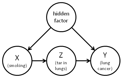
Statisticians like to use the example of smoking and lung cancer. We can borrow a causal diagram like the one above (hat tip to Michael Nielsen for this diagram). The goal of causal discovery is to determine this entire causal diagram: given all the nodes (variables), which edges (correlations) exist? and which are explained away once we know the other variables? For example, we want to know if $X$ (smoking) really causes $Y$ (lung cancer), or if there is a hidden factor (perhaps genetics) that is confounding the relationship. Or if there is even no residual correlation between $X$ and $Y$.

The core idea of causal discovery is that different causal structures produce different independence relationships. And independence relationships are things that you can determine from the data itself. For example, if A -> B -> C is the true causal diagram, then if we condition on B, there should be NO correlation between A and C (they should be independent). The core idea is to exploit conditional independence tests and infer the causal graph structure from these tests. If you make the right assumptions, you can recover the causal structure of the system. There are a number of algorithms to compute causal structures given independent samples from a data generating function. But we're going to look at one of the most robust ones that exploits time series data.

PCMCI Algorithm

In a series of papers, Jakob Runge and colleagues developed the PCMCI algorithm. The algorithm is an extension of the PC algorithm (named after Peters and Clark) and first published here, which recovers the graphical structure of a data set without exploiting time series information. The main benefit of PCMCI is that it exploits massive time series data to get a more powerful view of the causal structure of a time-dependent system.

General Setup

The general setup is an underlying time-dependent system: $\mathbf{X}_t = (X_t^1, ... X_t^N)$, where

$X_t^j = f_j(\mathcal{P}(X_t^j), \eta_t^j)$

This setup means that each of the $j$ variables at time $t$ (i.e., $X_t^j$ ) is a function ($f_j$) of its parents, $\mathcal{P}(X_t^j)$, and a noise term , $\eta_t^j$. The function is unique for each $j$ variable because the function is indexed for each variable ($f_j$). This function can have any functional form, and can even be non-linear.

This is a very general setup! It includes most of the causal questions we're interested in across all scientific fields, such as "What is causing high unemployment?", "What has caused an increase in 'deaths of despair' in America?", "What are the causes of global warming?", and "What is the cause of congestion in a traffic system?". I'm pretty hard-pressed to find a process that would NOT fall under this setup! Possibilities include:

• Completely deterministic systems where there is no noise term. Could this setup account for deterministic systems by just making the error term very small or even non-existent? It's unclear to me if the error term is required by either the PC or the MCI steps of the algorithm (more on these later). It's possible that the conditional independence tests in the MCI step would fail because they rely on checking correlations between two residuals from a regression. If a system is completely deterministic, there would be no residuals, and the test would try to correlate two vectors of 0's (and when the standard deviation is 0, then a standard Pearson correlation test will fail).
• Dynamically coupled systems, such as systems in predator-prey population dynamics might not fall within this setup. I'm thinking of Sugihara et al. 2012. I can't remember if these dynamically coupled systems have no error terms. Could this setup account for that by having a very small error term?
• Complete random walks / Brownian noise, where the noise term dominates the system. But I think in this case, the parents of each variable ($\mathcal{P}(X_t^j)$) would just be an empty set, and the error term would dominate.
• Non-time-series systems, where we only have measurement at a single time point. If we only have a measurement of a system at a single time point, perhaps even after a randomized intervention, we would not be able to use the model in this setup. To clarify, the system is not the limiting factor here. Instead, our measurement of that system is limiting our use of this framework.

Alternative Graph Formulation

This system can also be represented as a graph:

$G = (\textbf{X} \times \mathbb{Z}, E)$

where $G$ is the graph, $\textbf{X}$ is a multivariate discrete-time stochastic process, and time is indexed by $t \in \mathbb{Z}$ (which explains why the graph is $\textbf{X} \times \mathbb{Z}$).

In this graph, the vertices are the variables, and the edges represent the causal structure.

There is some data-generating process that is time-dependent:

$X_t^j = f_j(\mathcal{P}(X_t^j), \eta_t^j), j \in {1,...,N}$

where $j$ indexes the variables in $\textbf{X}$, and $t$ indexes time lags.

The possible parents of a variable are all variables at all previous time points (this excludes the present): $\mathcal{P}(X_t^j)\subset \textbf{X}^{-}_t$, where $\textbf{X}^{-}= (\textbf{X}_{t-1}$, $\textbf{X}_{t-2}, ...)$. This means that the possible causal parents of variable $X_t^j$ are all the previous values of $\textbf{X}^{-}_t$. The goal is to determine which subset of these variables are the actual causal parents.

Assumptions

The PCMCI algorithm makes a number of assumptions. These are pretty restrictive:

1. Causal Sufficiency or Unconfoundedness: all common drivers of the causal process are observed. If you're familiar with Ordinary Least Squares (OLS), this is the standard assumption there.
2. Causal Markov Condition: $X_j^t$ is independent.

(I should probably unpack these assumptions more.)

Conditional Independence Tests

For each variable, we need a way to test if the set of candidate causal parents ($\hat{\mathcal{P}}(X_t^j)$) is in fact a true parent of the variable ($\mathcal{P}(X_t^j)$). The intuition is that if a variable is a parent of a child, then the parent will be correlated with the child, even after conditioning on all other variables. That's the very definition of causation: ever after accounting for all other variables, the parent has an effect on the child.

Mathematically, we need a general test for the following conditional independence relationship:

$X \perp \!\!\! \perp Y \enspace | \enspace \mathbf{Z}$

If this relationship holds, then we can say that $Y$ is a cause of $X$ (or vice versa), even after accounting for $Z$. Additionally, if $Y$ is temporally prior to $X$, then we can use that information to determine causal direction: we know $Y$ must be causing $X$.

And further, we need this test to be available for any type of functional forms $f(X, Y)$, where $f$ might be (1) linear in the inputs, (2) polynomial in the inputs, or (3) follow non-linearities with respect to the error terms of each variable, $\eta^X$ and $\eta^Y$.

Limitations. It is unclear to me if the current setup accounts for non-linearities in the function form, such as sharp thresholds like agent-based models of complex contagions (and review), or the indicator function, $\mathbb{1(\cdot)}$, or anything involving $>$ or $<$, as in the Rectified Linear Unit (ReLU).

1. Partial Correlation (ParCorr)

The Partial Correlation test is a residuals-based test based on running two linear regressions:

1. regress $Z$ ~ $X$ and store the residuals, $r_{z,x}$.
2. regress $Z$ ~ $Y$ and store the residuals, $r_{z,y}$.
3. conduct a correlation test (Pearson correlation?) on the two residuals, $r_{z,x}$ and $r_{z,y}$. If the p-value is not significantly different than 0 (based on the chosen $\alpha$ level), then you cannot reject the null hypothesis of no correlation. Otherwise, there is correlation, and we form an edge in the causal graph: we connect $X$ and $Y$ conditional on $Z$.

This test can only capture linear dependencies. For example, it fails to account for time-dependent processes such as the following:

$X = Z^2 + \eta^X$

Though, I guess you could build polynomial regressions when constructing the residuals (?).

2. Gaussian Process Regression + Distance Correlation (GPDC)

The main problem with using partial correlation on residuals from two linear regressions is that it cannot handle non-linear functional forms like $X = Z^2 + \eta^X$ and $Y = -Z^2 + \eta^Y$ for $Z \sim \mathcal{N} (0,1)$.

Gaussian Process Regression

Gaussian Process Regression, plus Distance Correlation (GP+DC) is another residual-based conditional independence test that handles non-linearities. It relies on replacing the linear regression in the ParCorr test above with a Gaussian Process (GP) regression. And the correlation test (Pearson correlation, above) is replaced with a distance correlation coefficient, based on a paper in the Annals of Statistics by Szekely, Rizzo, and Bakirov (2007).

Why GP regression? The main benefit of a GP regression is that it can capture any functional form. My understanding is that you could effectively replace the GP regression with a spline or any other flexible curve-fitting algorithm. The only thing that differs is that GP (or at least kriging, according to Wikipedia) gives the Best Linear Unbiased Estimator of the intermediate values (i.e., the values for which we do not have a point already in the training set). [Side note: this confuses me b/c GP does not appear to be a linear estimator at all.] The justification mentioned in the paper is that GP is:

1. Bayesian (which is a natural way to justify a method), and
2. non-parametric (which is also always nice to claim).

I guess #1 is the main difference between using GP and using splines or some other curve fitting method. Though I don't completely understand this choice.

There is a helpful intro to Gaussian Process Regression here, and the Wikipedia article on kriging has me believe that it is nothing more than a kind of spline that can flexibly handle any functional form. Additionally, there are the 2 benefits mentioned above.

Distance Correlation

Distance correlation is confusing, and the paper on it is a mathematical morass [paper]. In the absence of understanding it, let's use mental heuristics: it's popular, and cited by 1275 articles.

The main benefit of distance correlation is that it ranges between 0 and 1, and is 0 if and only if the variables are independent. Further, distance correlation measures linear and non-linear association. [Side note: this is confusing to me because I thought the purpose of GP regression was to capture the non-linear relations among variables. If GP regression successfully did this, then the residuals should just be white noise—at least that's my assumption. The implication appears to be that even if GP regression captures non-linear relations, the residuals will be non-linear, and Pearson correlation will fail to capture the relationship.]

3. Conditional Mutual Information (CMI)

The main limitation of any 2-step procedure for estimating conditional independence (which includes Partial Correlation and GP+DC) is that it assumes additive noise.

What is an example of a function that would not work with the above tests?

$X = Z \cdot \eta^X$

$Y = Z \cdot \eta^Y$

In this example, the error terms specific to $X$ and $Y$, $\eta^X$ and $\eta^Y$, changes at different levels of another variable, $Z$.

[Side note: This raises an interesting definitional question as to what non-linear actually means. The paper seems to use it in the sense of non-linear additive. It's important to specify the additive part.]

Key Idea. The key idea of Conditional Mutual Information (CMI) is that it is a measure of mutual information, conditional on some other information. In general, conditional mutual information is defined as:

$I(X;Y|Z) = \int\int\int p(x,y,z) \cdot log \frac{p(x,y|z)}{p(x|z) \cdot p(y|z)} \cdot dx \cdot dy \cdot dz$

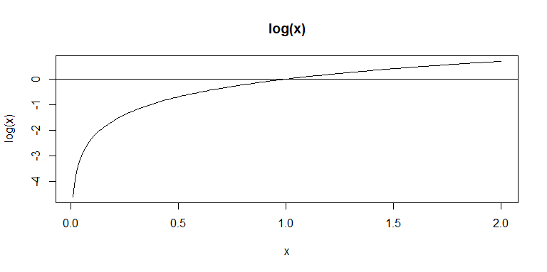
What does this mean? Remember that the $log(\frac{1}{bignumber}) \rightarrow -\infty$, and $log(1)=0$, and that $log(>1)$ increases slowly. The $log(\cdot)$ part of this function will only be 0 when the numerator and denominator are equal. And that only occurs when $x$ and $y$ are independent (conditional on $z$, of course). Recall, the very definition of independence is that the joint distribution equals the product of the two marginals:

$p(x,y)=p(x) \cdot p(y).$

[Side note: I'm confused because my recollection of mutual information is that it is not transitive, that is $I(X;Y) \neq I(Y;X)$.

Note: this is only defined for continuous variables (because of the integral over the joint density). I think it's possible to substitute the integral for a summation, and I believe that's what the tigramite package does.

Extensions

Mechanisms and the meaning of "causation". Causation in this framework has a strange meaning. I'm reminded of the hand-waving, and scare-quotes you always see around "Granger causation" versus just causation, simpliciter. What I mean is that it's unclear that this method will be able to reveal the mechanism of a complex system, even if it can identify the variables that "cause" each other. (Separately, it would be really interesting if it could propose and test an agent-based model capable of reproducing the time-series dynamics.) Also, this method would appear to provide different results at different levels of temporal aggregation. In my experience on using this method with time series data of different temporal granularities (5-mins, hourly, and daily), you see very different causal patterns. Maybe we can resolve this, and it is fundamentally no different than saying "temperature causes $X$" (i.e., average molecular motion over a volume causes $X$), when at a more fine-grained temporal and spatial analysis, there are really all these complex collisions that are the real causes.